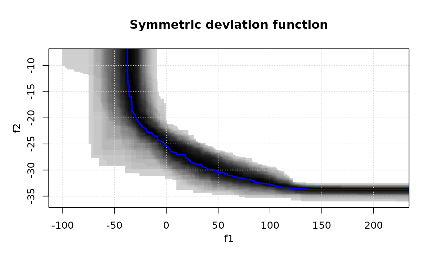
Compute Vorob'ev threshold, expectation and deviation. Also, displaying the symmetric deviation function is possible. The symmetric deviation function is the probability for a given target in the objective space to belong to the symmetric difference between the Vorob'ev expectation and a realization of the (random) attained set.
Arguments
- x
Either a matrix of data values, or a data frame, or a list of data frames of exactly three columns. The third column gives the set (run, sample, ...) identifier.
- reference
(
numeric())
Reference point as a vector of numerical values.- VE, threshold
Vorob'ev expectation and threshold, e.g., as returned by
vorobT().- nlevels
number of levels in which is divided the range of the symmetric deviation.
- ve.col
plotting parameters for the Vorob'ev expectation.
- xlim, ylim, main
Graphical parameters, see
plot.default().- legend.pos
the position of the legend, see
legend(). A value of"none"hides the legend.- col.fun
function that creates a vector of
ncolors, seeheat.colors().
Value
vorobT returns a list with elements threshold,
VE, and avg_hyp (average hypervolume)
vorobDev returns the Vorob'ev deviation.
References
BinGinRou2015gaupareaf
C. Chevalier (2013), Fast uncertainty reduction strategies relying on Gaussian process models, University of Bern, PhD thesis.
I. Molchanov (2005), Theory of random sets, Springer.
Examples
data(CPFs)
res <- vorobT(CPFs, reference = c(2, 200))
print(res$threshold)
#> [1] 44.14062
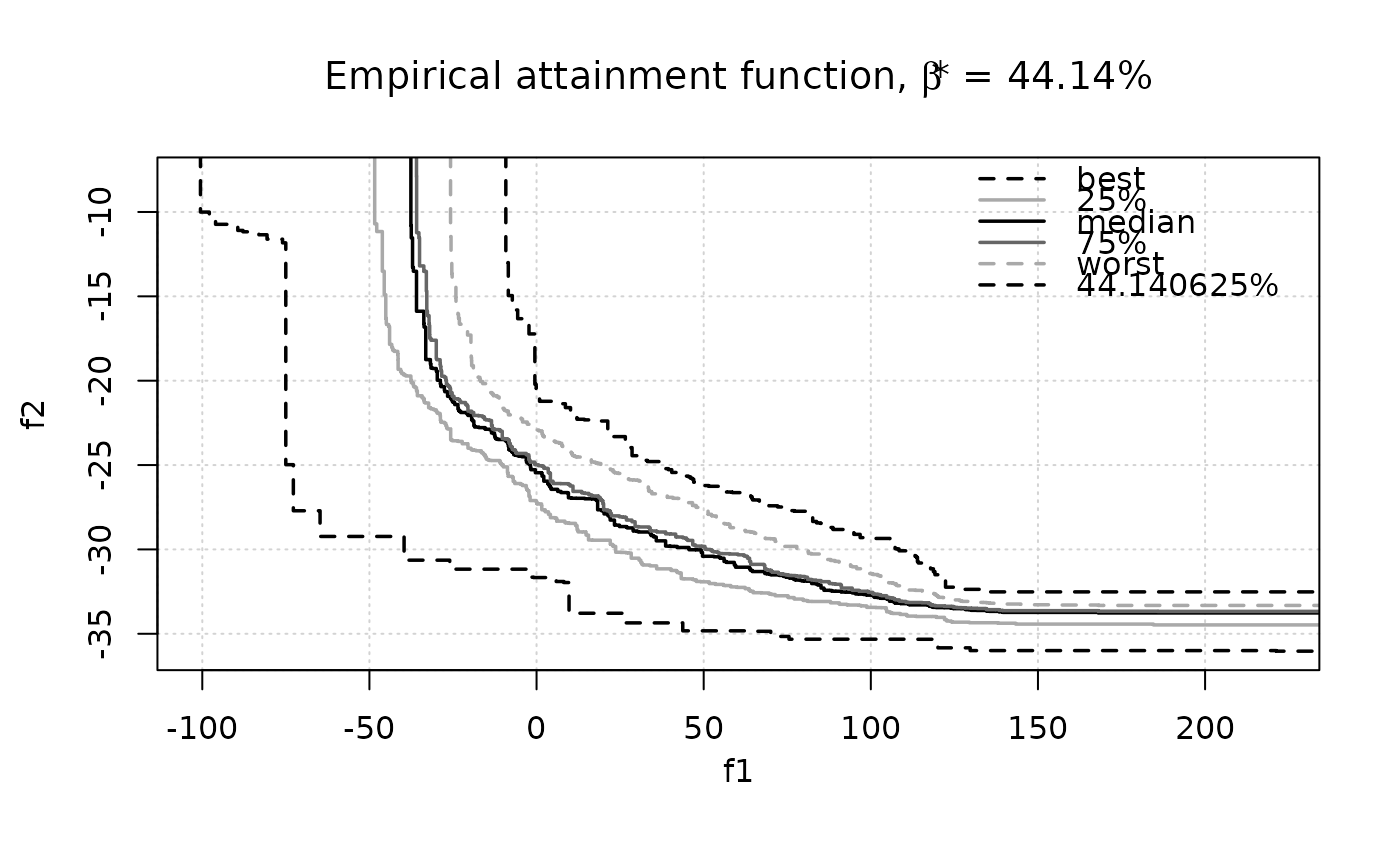
## Display Vorob'ev expectation and attainment function
# First style
eafplot(CPFs[,1:2], sets = CPFs[,3], percentiles = c(0, 25, 50, 75, 100, res$threshold),
main = substitute(paste("Empirical attainment function, ",beta,"* = ", a, "%"),
list(a = formatC(res$threshold, digits = 2, format = "f"))))
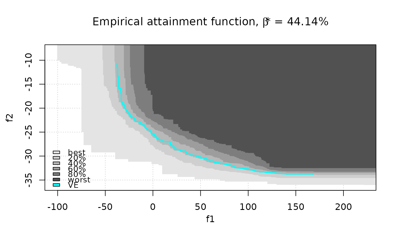
 # Second style
eafplot(CPFs[,1:2], sets = CPFs[,3], percentiles = c(0, 20, 40, 60, 80, 100),
col = gray(seq(0.8, 0.1, length.out = 6)^0.5), type = "area",
legend.pos = "bottomleft", extra.points = res$VE, extra.col = "cyan",
extra.legend = "VE", extra.lty = "solid", extra.pch = NA, extra.lwd = 2,
main = substitute(paste("Empirical attainment function, ",beta,"* = ", a, "%"),
list(a = formatC(res$threshold, digits = 2, format = "f"))))
# Second style
eafplot(CPFs[,1:2], sets = CPFs[,3], percentiles = c(0, 20, 40, 60, 80, 100),
col = gray(seq(0.8, 0.1, length.out = 6)^0.5), type = "area",
legend.pos = "bottomleft", extra.points = res$VE, extra.col = "cyan",
extra.legend = "VE", extra.lty = "solid", extra.pch = NA, extra.lwd = 2,
main = substitute(paste("Empirical attainment function, ",beta,"* = ", a, "%"),
list(a = formatC(res$threshold, digits = 2, format = "f"))))
 # Now print Vorob'ev deviation
VD <- vorobDev(CPFs, res$VE, reference = c(2, 200))
print(VD)
#> [1] 3017.13
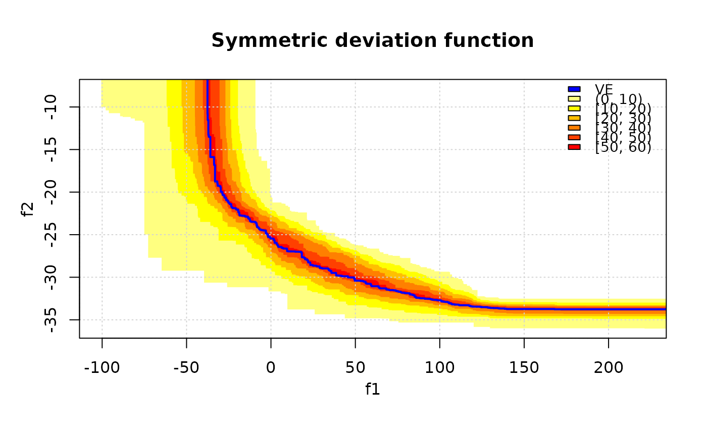
# Now display the symmetric deviation function.
symDifPlot(CPFs, res$VE, res$threshold, nlevels = 11)
# Now print Vorob'ev deviation
VD <- vorobDev(CPFs, res$VE, reference = c(2, 200))
print(VD)
#> [1] 3017.13
# Now display the symmetric deviation function.
symDifPlot(CPFs, res$VE, res$threshold, nlevels = 11)
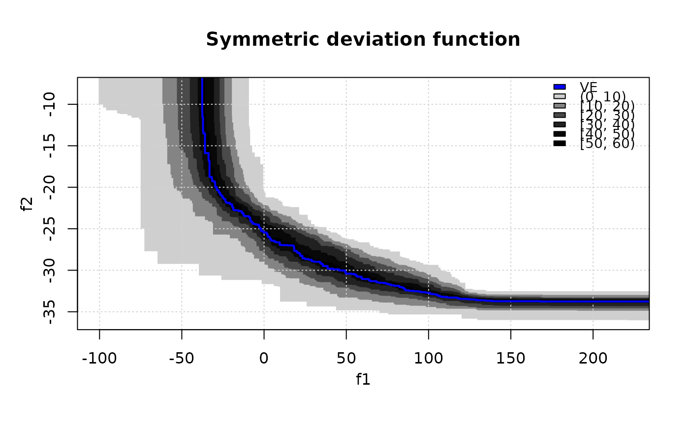 # Levels are adjusted automatically if too large.
symDifPlot(CPFs, res$VE, res$threshold, nlevels = 200, legend.pos = "none")
# Levels are adjusted automatically if too large.
symDifPlot(CPFs, res$VE, res$threshold, nlevels = 200, legend.pos = "none")
 # Use a different palette.
symDifPlot(CPFs, res$VE, res$threshold, nlevels = 11, col.fun = heat.colors)
# Use a different palette.
symDifPlot(CPFs, res$VE, res$threshold, nlevels = 11, col.fun = heat.colors)