Computation and visualization of the empirical attainment function (EAF) for the analysis of random sets in multi-criterion optimization.

The empirical attainment function (EAF) describes the probabilistic distribution of the outcomes obtained by a stochastic algorithm in the objective space. This package implements plots of summary attainment surfaces and differences between the first-order EAFs. These plots may be used for exploring the performance of stochastic local search algorithms for biobjective optimization problems and help in identifying certain algorithmic behaviors in a graphical way.

Functions

eafdiffplot()	Empirical attainment function differences
eafplot()	Plot the Empirical Attainment Function for two objectives
read_datasets()	Read several data.frame sets

Data

gcp2x2

Metaheuristics for solving the Graph Vertex Coloring Problem

HybridGA

Results of Hybrid GA on vanzyl and Richmond water networks

SPEA2minstoptimeRichmond

Results of SPEA2 when minimising electrical cost and maximising the minimum idle time of pumps on Richmond water network

Extras are available at system.file(package="eaf"):

extdata	External data sets (see read_datasets)
scripts/eaf	EAF command-line program
scripts/eafplot	Perl script to generate plots of attainment surfaces
scripts/eafdiff	Perl script to generate plots of EAF differences

References

Grunert01eaf

GruFon2009:emaaeaf

LopPaqStu09emaaeaf

FonGueLopPaq2011emoeaf

See also

Useful links:

• https://mlopez-ibanez.github.io/eaf/

• https://github.com/MLopez-Ibanez/eaf

• Report bugs at https://github.com/MLopez-Ibanez/eaf/issues

Author

Maintainer: Manuel López-Ibáñez manuel.lopez-ibanez@manchester.ac.uk (ORCID)

Authors:

• Marco Chiarandini

• Carlos Fonseca

• Luís Paquete

• Thomas Stützle

Other contributors:

• Mickaël Binois [contributor]

Examples

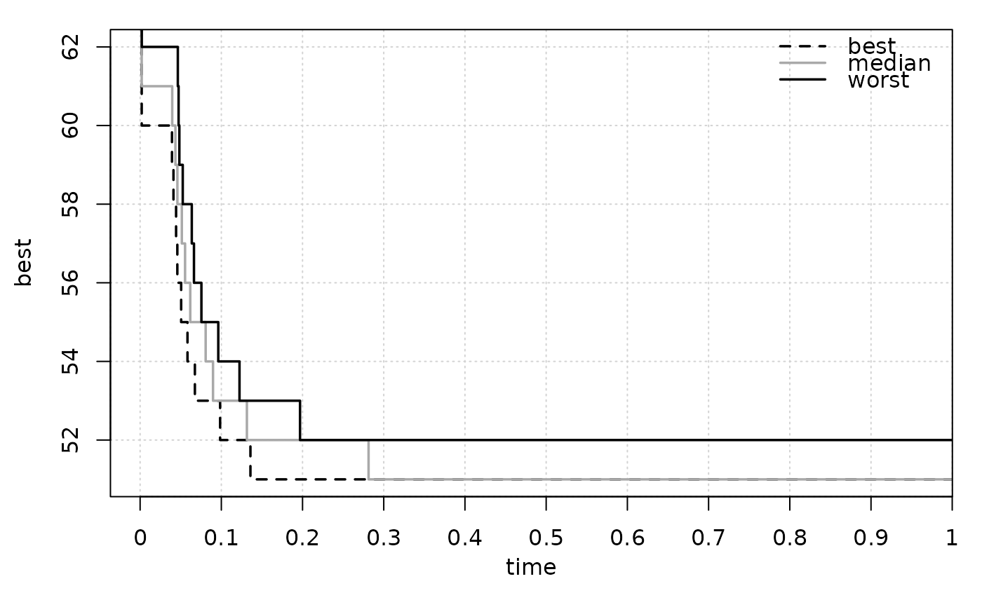
data(gcp2x2)
tabucol<-subset(gcp2x2, alg!="TSinN1")
tabucol$alg<-tabucol$alg[drop=TRUE]
eafplot(time+best~run,data=tabucol,subset=tabucol$inst=="DSJC500.5")


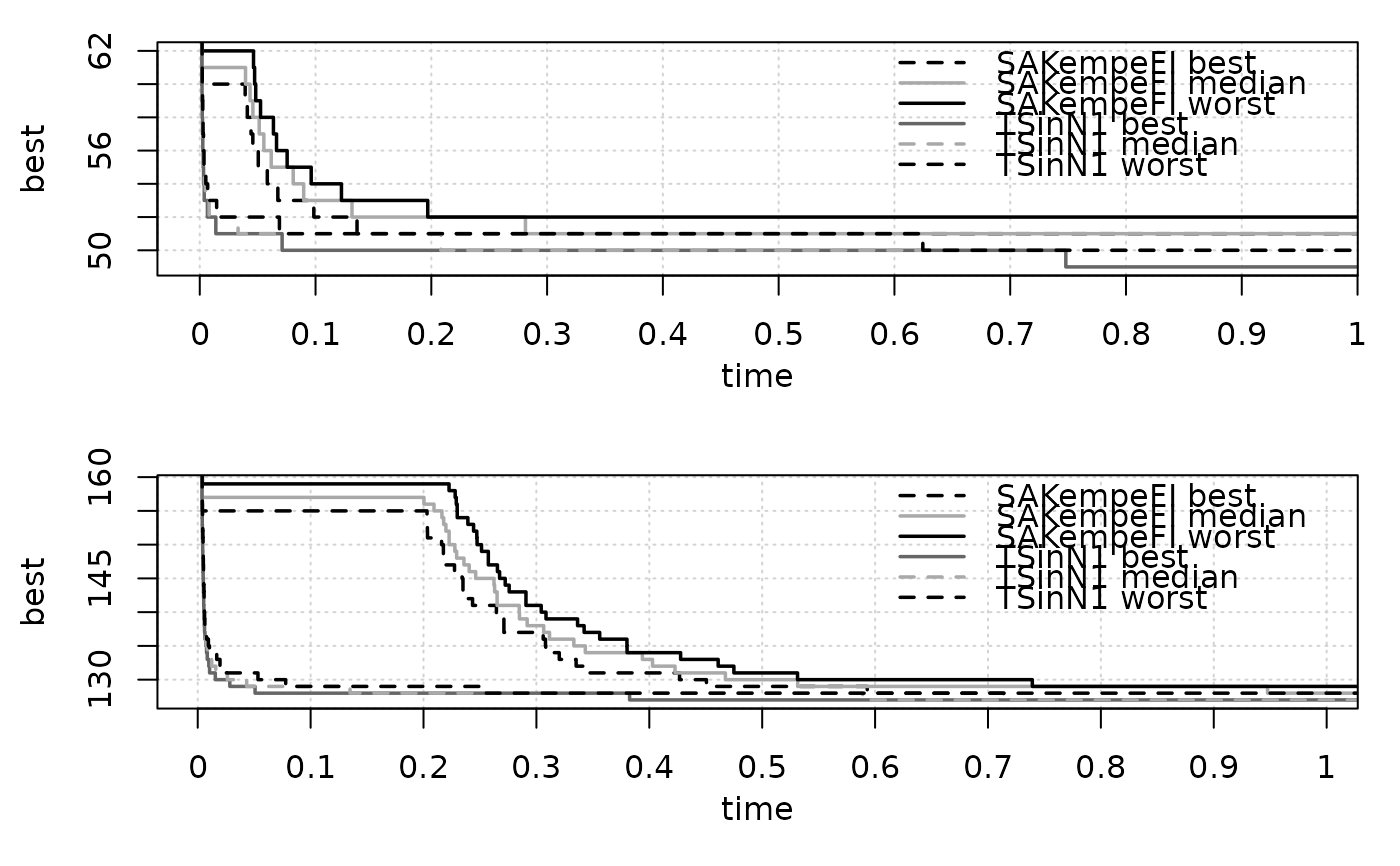
eafplot(time+best~run|inst,groups=alg,data=gcp2x2)

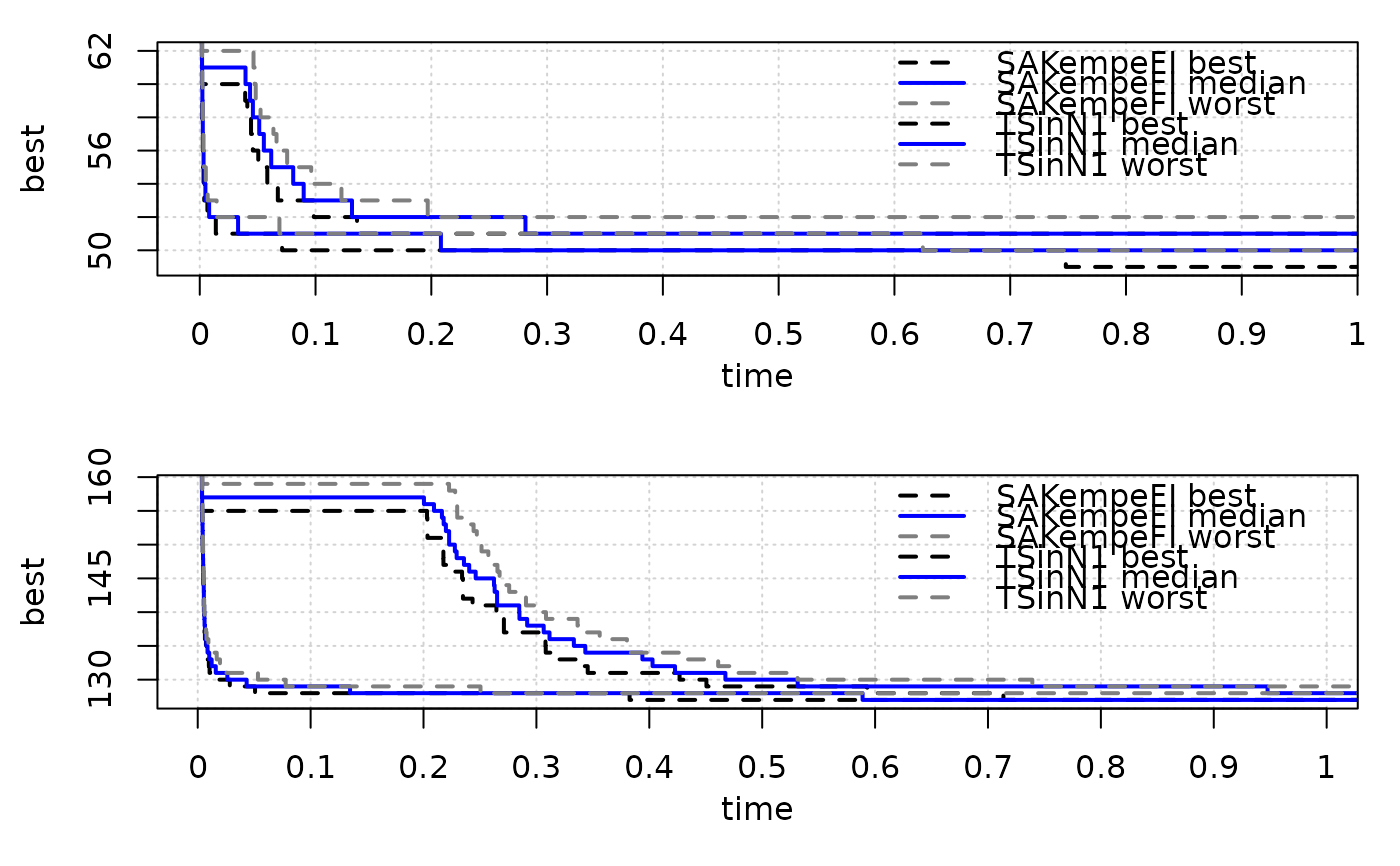
eafplot(time+best~run|inst,groups=alg,data=gcp2x2,
  percentiles = c(0,50,100), cex = 1.4, lty = c(2,1,2),lwd = c(2,2,2),
        col = c("black","blue","grey50"))

 
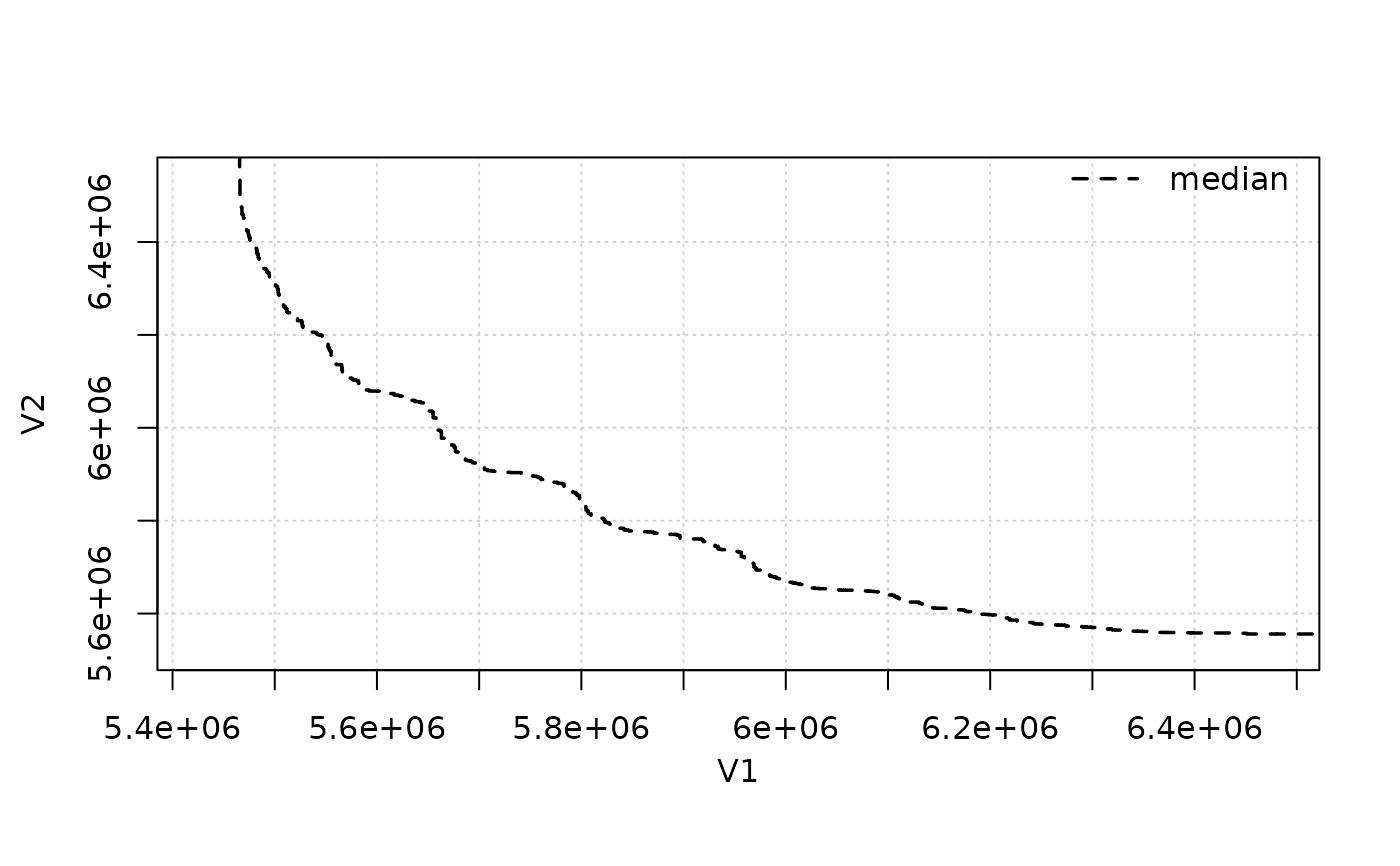
extdata_path <- system.file(package="eaf","extdata")
A1 <- read_datasets(file.path(extdata_path, "wrots_l100w10_dat"))
A2 <- read_datasets(file.path(extdata_path, "wrots_l10w100_dat"))
eafplot(A1, percentiles=c(50))

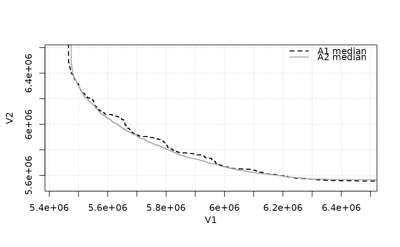
eafplot(list(A1=A1, A2=A2), percentiles=c(50))

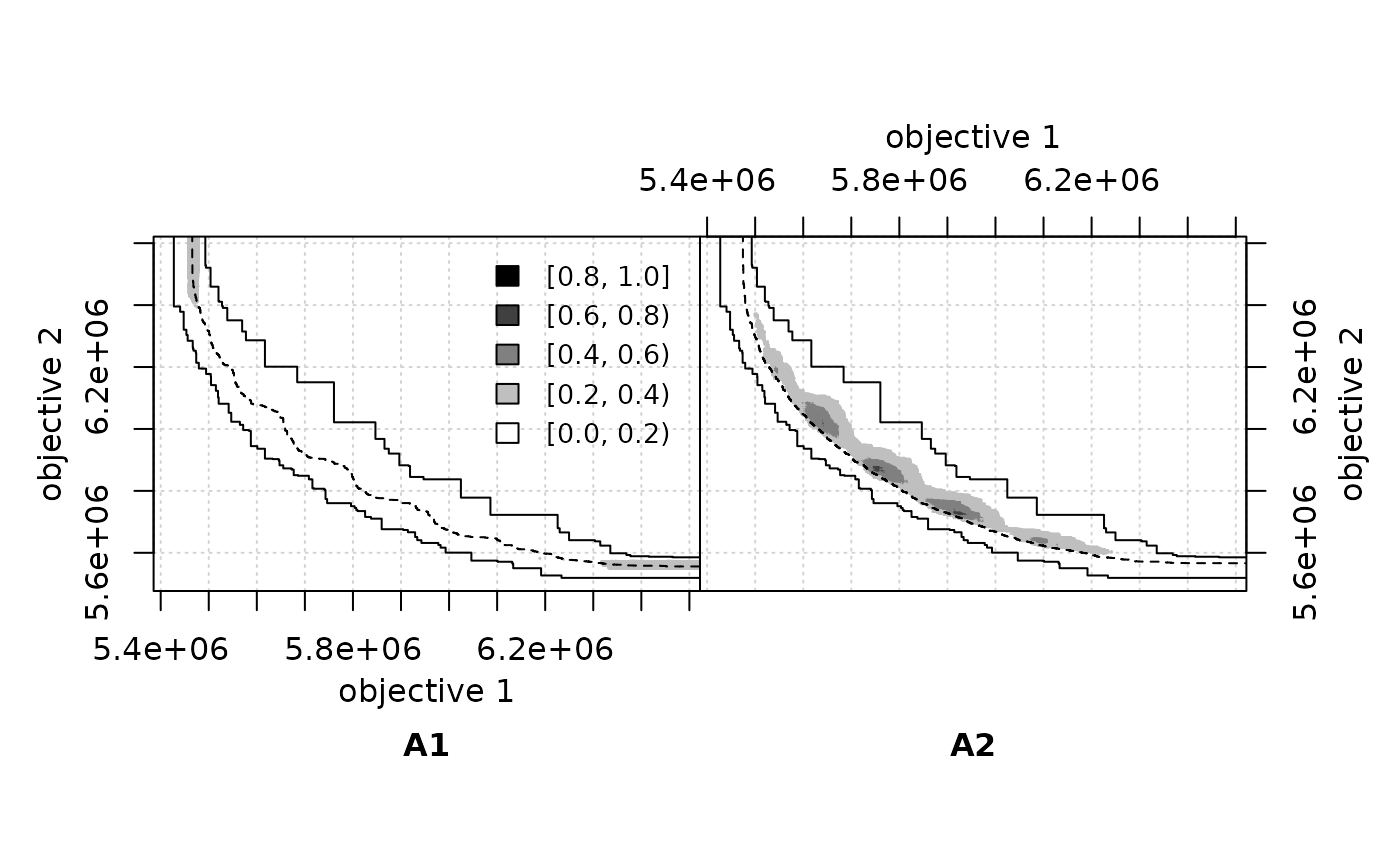
eafdiffplot(A1, A2)

## Save to a PDF file
# dev.copy2pdf(file="eaf.pdf", onefile=TRUE, width=5, height=4)